Experiment 8 $e / m$ of the Electron 实验8 电子的 $e / m$

1 Purpose 1 目的

In this experiment, you will measure the charge to mass ratio of the electron, a quantity known as $\mathrm{e} / \mathrm{m}$. The procedure demonstrates how we can use fairly basic equipment to observe one of the fundamental constituents of matter.

在本实验中，你将测量电子的电荷质量比，这个量被称为$\mathrm{e} / \mathrm{m}$。该实验过程展示了我们如何使用基本的设备来观察物质的基本组成部分之一。

2 Introduction 2 引言

The "discovery" of the electron by J.J. Thomson in 1897 refers to the experiment in which it was shown that "cathode rays" behave as beams of particles, all of which have the same ratio of charge to mass, $e / m$. At the time, Thomson correctly recognized that he had isolated a fundamental particle of nature; for his work, he won the Nobel Prize in 1906.

电子的"发现"是由J.J.汤姆森在1897年完成的，这项实验表明"阴极射线"表现为粒子束，所有粒子都具有相同的电荷质量比$e / m$。当时，汤姆森正确地认识到他发现了自然界的一个基本粒子；因为这项工作，他在1906年获得了诺贝尔奖。

Thomson's experiment, and the one we will conduct today, is a simple application of the motion of a charged particle in a magnetic field. Recall that if a particle of charge $e$ moves with velocity $\vec{v}$ into a region with some magnetic field $\vec{B}$, it will feel a magnetic deflection force

汤姆森的实验，以及我们今天要进行的实验，是带电粒子在磁场中运动的一个简单应用。回想一下，如果带电荷$e$的粒子以速度$\vec{v}$进入具有磁场$\vec{B}$的区域，它将受到磁偏转力

$$\begin{equation*} \vec{F}_{\text {mag }}=e \vec{v} \times \vec{B} \tag{8.1} \end{equation*}$$

Note the similarities between this expression and the magnetic force on a current-carrying wire: $\vec{F}_{\text {wire }}=i \vec{L} \times \vec{B}$. This equation is in fact just a generalization of the force on a point charge, since a current is nothing more than a flow of charge.

注意这个表达式与载流导线所受磁力的相似性：$\vec{F}_{\text {wire }}=i \vec{L} \times \vec{B}$。这个方程实际上只是点电荷所受力的推广，因为电流无非就是电荷的流动。

Consider the special case where $\vec{v}$ and $\vec{B}$ are perpendicular, and the magnitude of $\vec{B}$ is uniform. As shown in Fig. 8.1, the force $\vec{F}_{\text {mag }}$ is directed in such a way that the particle moves in a circle of radius $r$, with the plane of the circle perpendicular to $\vec{B}$.

考虑$\vec{v}$和$\vec{B}$垂直，且$\vec{B}$大小均匀的特殊情况。如图8.1所示，力$\vec{F}_{\text {mag }}$的方向使粒子在半径为$r$的圆周上运动，圆平面垂直于$\vec{B}$。

Since the particle moves in uniform circular motion, the magnetic force is a centripetal force,

由于粒子做匀速圆周运动，磁力就是向心力，

$$\begin{equation*} \vec{F}_{c}=m \frac{v^{2}}{r} \tag{8.2} \end{equation*}$$

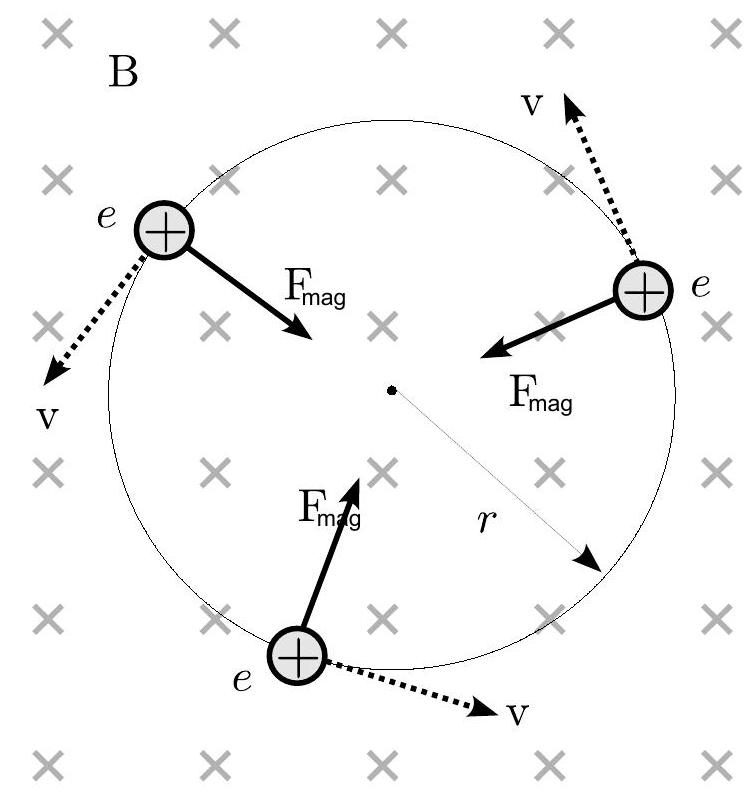
Figure 8.1: Deflection of a charged particle in a uniform field $\vec{B}$ directed into the page.

图8.1：带电粒子在指向纸内的均匀场$\vec{B}$中的偏转。

We can consider equations (8.1) and (8.2) for the special case where $\vec{v}$ and $\vec{B}$ are perpendicular, and the magnitude of $\vec{B}$ is uniform. They suggest that, in principle, if we could measure the incoming velocity $v$ of the particle, we could use this result to directly measure the charge to mass ratio $e / m$.

我们可以考虑$\vec{v}$和$\vec{B}$垂直且$\vec{B}$大小均匀的特殊情况下的方程(8.1)和(8.2)。这表明原则上如果我们能测量粒子的入射速度$v$，就可以用这个结果直接测量电荷质量比$e / m$。

In practice, direct measurements of $v$ are not feasible. However, if we use some known potential difference $V$ to accelerate the particle from rest to a speed $v$, we could rewrite the speed in terms of $V$ using energy conservation:

实际上，直接测量$v$是不可行的。但是，如果我们使用已知的电位差$V$将粒子从静止加速到速度$v$，我们可以用能量守恒用$V$来表示速度：

$$\begin{equation*} U_{k i n}=\frac{1}{2} m v^{2} \quad \text { and } \quad U_{p o t}=e V \tag{8.3} \end{equation*}$$

By substituting $v$ in equations (8.2) and (8.3), $e / m$ can be expressed directly in terms of $V, B$, and the easily observed radius of curvature $r$ :

通过在方程(8.2)和(8.3)中代入$v$，$e / m$可以直接用$V, B$和容易观测到的曲率半径$r$表示：

$$\begin{equation*} \frac{e}{m}=\frac{2 V}{B^{2} r^{2}} \tag{8.4} \end{equation*}$$

3 Experiment 3 实验

In the setup you will use, electrons are emitted at a very low velocity from a heated filament, accelerated through an electrical potential $V$ to a final velocity $v$, and finally bent in a circular path of radius $r$ in a magnetic field $B$. The entire process takes place in a sealed glass tube in which the path of the electrons can be directly observed. During its manufacture, the tube was evacuated and backfilled with a small trace of helium gas. When electrons in the beam have sufficiently high kinetic energies ( $\geq 10.4 \mathrm{eV}$ ), a small fraction of them will ionize helium atoms. Recombination of the helium ions, accompanied by the emission of a characteristic blue light, occurs very near the point where the ionization took place. As a result, the path of the electron beam is visible to the naked eye as a thin blue beam of light.

在你将使用的装置中，电子从加热的灯丝以很低的速度发射出来，通过电势$V$加速到最终速度$v$，最后在磁场$B$中沿半径为$r$的圆形路径弯曲。整个过程发生在密封的玻璃管中，其中电子的路径可以直接观察到。在制造过程中，管被抽真空并充入少量氦气。当束流中的电子具有足够高的动能（$\geq 10.4 \mathrm{eV}$）时，其中一小部分会电离氦原子。氦离子的复合过程伴随着特征蓝光的发射，发生在电离发生的位置附近。因此，电子束的路径在肉眼可见时呈现为一束细细的蓝光。

3.1 Electron Gun in Vacuum Tube 3.1 真空管中的电子枪

Figure 8.2 shows the indirectly heated cathode and the anode plate used to accelerate the electrons. The cathode is heated by passing a current directly through the heater. A variable positive potential difference of up to 500 V is then applied between the anode and the cathode in order to accelerate the electrons emitted from the cathode. Some of the accelerated electrons come out as a narrow beam through a small aperture on the grid.

图8.2展示了用于加速电子的间接加热阴极和阳极板。阴极通过直接通过加热器的电流加热。在阳极和阴极之间施加最高500 V的可变正电位差，以加速从阴极发射的电子。一些加速后的电子通过栅极上的小孔径形成窄束射出。

The tube is set up so that the beam of electrons travels perpendicular to a uniform magnetic field $B$, and is initially vertical. The $B$ field is produced by the current $I$ running through a pair of large diameter coils (so-called "Helmholtz coils") designed to produce optimum field uniformity near the center.

管的设置使电子束垂直于均匀磁场 $B$ 传播，初始方向为垂直向上。$B$ 场由通过一对大直径线圈（即所谓的"亥姆霍兹线圈"）的电流 $I$ 产生，这种设计可在中心区域产生最佳的场均匀性。

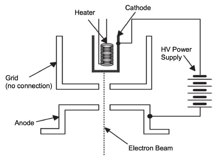
Figure 8.2: Diagram of the electron gun in the sealed glass tube.

图8.2：密封玻璃管中的电子枪示意图。

3.2 The Helmholtz Coils and the Uniform Magnetic Field # 3.2 亥姆霍兹线圈和均匀磁场

A current $I$ flowing in a single loop of wire of radius $R$ produces a magnetic field on the symmetry axis given by:

半径为 $R$ 的单圈导线中流过电流 $I$ 在对称轴上产生的磁场由下式给出：

$$B_{\text {loop }}=\frac{\mu_{0} R^{2} I}{2\left(R^{2}+x^{2}\right)^{3 / 2}}$$

$x$ is the distance from the plane of the loop. The electromagnet used in this experiment, shown in Fig. 8.3, consists of two loops of wire with $N$ turns each, separated by a distance $R$ (the same $R$ as the coil radius). The coils contribute equally to the field at the center ( $x=R / 2$ ), so at that point

$x$ 是从线圈平面的距离。本实验中使用的电磁铁如图8.3所示，由两个各有 $N$ 匝的导线环组成，间距为 $R$（与线圈半径相同的 $R$）。这些线圈在中心点（$x=R / 2$）对场的贡献相等，因此在该点：

$$\begin{equation*} B_{I}=\frac{\mu_{0} R^{2} N I}{\left(R^{2}+(R / 2)^{2}\right)^{3 / 2}}=\left(\frac{4 \pi \times 10^{-7} N}{R(1+1 / 4)^{3 / 2}}\right) I=C \cdot I \tag{8.5} \end{equation*}$$

The setup in the laboratory has $N=132$ turns per coil, where each coil has a radius $R=0.1475 \mathrm{~m}$; before you come to the lab, use these numbers to calculate the constant $C$ (units of $\mathrm{T}^{-1}$ ). This arrangement, called a pair of Helmholtz coils, yields a highly uniform field in the region at the center.

实验室的装置每个线圈有 $N=132$ 匝，每个线圈的半径为 $R=0.1475 \mathrm{~m}$；在来实验室之前，使用这些数值计算常数 $C$（单位为 $\mathrm{T}^{-1}$）。这种称为亥姆霍兹线圈对的装置在中心区域产生高度均匀的场。

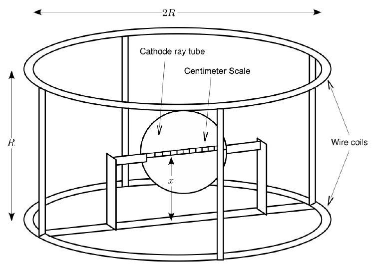
Figure 8.3: Helmholtz coils used to produce a uniform magnetic field.

图8.3：用于产生均匀磁场的亥姆霍兹线圈。

3.3 Estimating the Charge to Mass Ratio # 3.3 估算电荷与质量比

The electrons are therefore emitted into a region where a uniform magnetic field acts perpendicular to the motion of the electrons. The magnitude of the magnetic field can be adjusted until the resultant circular path of the electron beam just reaches the far end of the centimeter scale. The scale extends from the electron gun in a direction perpendicular to that in which the electron beam was emitted i.e., along a diameter of the circular orbits. The scale numbers on the scale fluoresce when struck by the electron beam. Then for given values of $V, B$ and $r$ it would be possible to determine $e / m$ from eq. (8.4).

因此，电子被发射到一个均匀磁场垂直于电子运动方向的区域。可以调节磁场的大小，直到电子束的圆形轨迹恰好到达厘米刻度的远端。刻度从电子枪开始延伸，方向垂直于电子束发射的方向，即沿着圆形轨道的直径。当电子束击中刻度时，刻度数字会发光。这样，对于给定的 $V, B$ 和 $r$ 值，就可以从方程(8.4)确定 $e / m$。

However, the net field $\vec{B}$ in which the electrons move is not only due to the Helmholtz coils, but also to the magnetic field in the ambient environment $\vec{B}_{E}$. A part of the ambient magnetic field is due to the Earth's magnetic field, but there may also be contributions from nearby ferromagnetic materials in the lab. Hence, the total field inside is the vector sum of $\vec{B}_{I}$ and $\vec{B}_{E}$. We can minimize the effect of $\vec{B}_{E}$ by aligning the $\vec{B}_{I}$ field with the direction of the needle of a compass close to the setup. The horizontal component of $\vec{B}_{E}$ is now aligned with $\vec{B}_{I}$. In fact, the value of $\vec{B}_{E}$ is so small that we can safely ignore it for the purpose of this lab. Incorporating eq. (8.5) into eq. (8.4) and rearranging terms, we obtain

然而，电子运动所在的净场 $\vec{B}$ 不仅来自亥姆霍兹线圈，还来自环境中的磁场 $\vec{B}_{E}$。环境磁场的一部分来自地球磁场，但实验室中附近的铁磁材料也可能有贡献。因此，内部的总场是 $\vec{B}_{I}$ 和 $\vec{B}_{E}$ 的矢量和。我们可以通过将 $\vec{B}_{I}$ 场与装置附近的指南针指针方向对齐来最小化 $\vec{B}_{E}$ 的影响。$\vec{B}_{E}$ 的水平分量现在与 $\vec{B}_{I}$ 对齐。实际上，$\vec{B}_{E}$ 的值很小，在本实验中可以安全地忽略它。将方程(8.5)代入方程(8.4)并重新整理项，我们得到

$$\begin{equation*} I \simeq\left(\frac{1}{C} \sqrt{\frac{2 V}{e / m}}\right) \frac{1}{r} \tag{8.6} \end{equation*}$$

Now, instead of performing a single measurement of $r$, we can measure the variation of $r$ with $B$ (or $I$ ) at fixed values of $V$, and use the fact that the coil current $I$ is a linear function of the curvature $1 / r$.

现在，我们不用进行单次 $r$ 的测量，而是可以在固定的 $V$ 值下测量 $r$ 随 $B$（或 $I$）的变化，并利用线圈电流 $I$ 是曲率 $1/r$ 的线性函数这一事实。

Note that eqs. (8.2), (8.3), and (8.6) apply only to electrons with trajectories on the outside edge of the beam - i.e., the most energetic electrons. This is because some electrons in the beam will lose energy through collisions with helium atoms.

注意方程(8.2)、(8.3)和(8.6)仅适用于在束流外边缘轨道上的电子——即最有能量的电子。这是因为束流中的一些电子会通过与氦原子的碰撞损失能量。

4 Procedure # 4 实验步骤 4.1 Derivations # 4.1 推导

Before you begin taking data, derive equations (8.4) and (8.6) using the concepts and basic assumptions described in the Introduction.

在开始收集数据之前，使用引言中描述的概念和基本假设推导方程(8.4)和(8.6)。

Check your work with your TA. When you write your lab report, you should include relevant equations from your derivation in your "Introduction" and "Methods" sections. Recall that your lab report should be clear and concise, so you should not include the full derivation in your report.

与你的助教核对你的工作。当你撰写实验报告时，你应该在"引言"和"方法"部分包含推导中的相关方程。记住你的实验报告应该清晰简洁，所以不应该在报告中包含完整的推导过程。

4.2 Orientation of the Coil and Tube Setup # 4.2 线圈和管装置的定向

For reasons already explained, we would like to orient the Helmholtz coils such that their axes are parallel to the horizontal direction of the ambient magnetic field. To do this,

出于已经解释过的原因，我们希望将亥姆霍兹线圈定向，使其轴线与环境磁场的水平方向平行。为此，

• Make sure that the setup is turned off before doing anything.
• Put a compass on the desk at a place close to the setup. Wait for the needle to stabilize.
• Rotate the setup such that the axes of the coils are parallel to the needle of the compass.
• The coil axis should now be aligned with the horizontal component of the ambient magnetic field.
• 在做任何事情之前，确保装置处于关闭状态。
• 在靠近装置的桌面上放置一个指南针。等待指针稳定。
• 旋转装置，使线圈的轴线与指南针的指针平行。
• 线圈轴线现在应该与环境磁场的水平分量对齐。

An example is shown in Fig. 8.4 Please exercise caution as you align the Helmholtz coils: the cathode ray tube is very delicate and may break if a large force is applied to it. It is recommended that you never touch the tube or the coils, and only maneuver the setup by touching the base.

一个示例如图8.4所示。 在对准亥姆霍兹线圈时请务必小心：阴极射线管非常脆弱，如果施加较大的力可能会破损。建议你永远不要触摸管或线圈，只能通过触摸底座来操作装置。

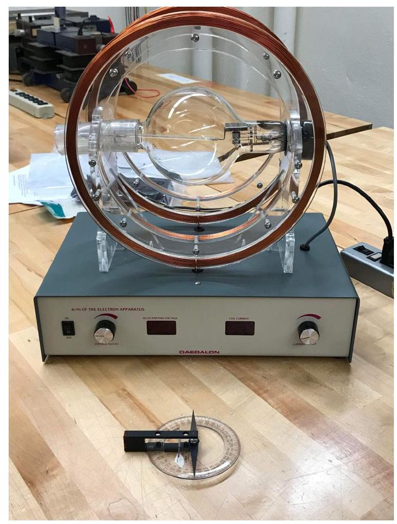
Figure 8.4: Example of the Helmholtz coils aligned to the ambient field.

图8.4：亥姆霍兹线圈与环境场对齐的示例。

4.3 Measurement of the Circular Orbits # 4.3 圆形轨道的测量

Once you are done with the alignment, you can turn on the setup and start taking data. Make sure only the dim incandescent ceiling lights in the room are on.

完成对准后，你可以打开装置并开始收集数据。确保房间里只开启昏暗的白炽天花板灯。

• Turn on the power switch. The unit will perform a 30-second self-test, indicated by the digital display changing values rapidly. During the self-test, the controls are locked out, allowing the cathode to heat to the proper operating temperature. When the self-test is complete, the display will stabilize and show "000". Although the unit is now ready for operation, a 5-10-minute warm-up time is recommended before taking careful measurements.
• Turn the Voltage Adjust control up to 200 V and observe the bottom of the electron gun. The bluish beam will be travelling straight down to the envelope of the tube.
• Turn the Current Adjust control up and observe the circular deflection of the beam. When the current is high enough, the beam will form a complete circle within the envelope. The diameter of the beam can be measured using the internal centimeter scale inside of the tube. The scale numbers fluoresce when struck by the electron beam.
• For an accelerating voltage of 200 V, measure the beam diameter for a series of coil current settings. Alternatively, determine the coil current necessary to bring the beam to each prescribed distance on the tube arm. If the mark falls between steps on the ammeter, interpolate the current.
• Repeat the measurements for additional accelerating voltages: $300 \mathrm{~V}, 400 \mathrm{~V}$, and 500 V. Note that both the voltage and current outputs are controlled by an on-board microprocessor, which locks out the controls at both the minimum and maximum settings. The range for the voltage $V$ is $100-500 \mathrm{~V}$, while the range for the current $I$ is $1-3.0 \mathrm{~A}$.
• When all of the data has been collected, switch off the apparatus.
• 打开电源开关。设备将进行30秒的自检，通过数字显示快速变化的数值来指示。在自检期间，控制被锁定，允许阴极加热到适当的工作温度。当自检完成时，显示将稳定并显示"000"。虽然此时设备已经可以操作，但在进行仔细测量之前建议预热5-10分钟。
• 将电压调节控制调至200 V，观察电子枪底部。蓝色的束流将直接向下射向管的包络。
• 调高电流调节控制并观察束流的圆形偏转。当电流足够高时，束流将在包络内形成完整的圆。可以使用管内部的厘米刻度测量束流的直径。当电子束击中刻度时，刻度数字会发光。
• 在200 V的加速电压下，测量一系列线圈电流设置下的束流直径。或者，确定使束流到达管臂上每个规定距离所需的线圈电流。如果标记落在电流表的刻度之间，则对电流进行插值。
• 对其他加速电压重复测量：$300 \mathrm{~V}、400 \mathrm{~V}$和500 V。注意电压和电流输出都由板载微处理器控制，该处理器在最小和最大设置处锁定控制。电压$V$的范围是$100-500 \mathrm{~V}$，而电流$I$的范围是$1-3.0 \mathrm{~A}$。
• 当所有数据收集完毕后，关闭装置。

4.4 Summary of data: # 4.4 数据总结：

• $I$ and $r$ for four or five values of $V$
• Derivations for equations (8.4) and (8.6)
• 四个或五个 $V$ 值对应的 $I$ 和 $r$
• 方程(8.4)和(8.6)的推导

5 Analysis # 5 分析

When you finish the lab, you should have a data table for each accelerating voltage $V$ you used. The tables will contain values of $I$ as a function of $r$. To determine the charge to mass ratio $e / m$, you will plot $I$ versus $1 / r$ and perform the usual linear least squares analysis on the data.

当你完成实验后，你应该有每个使用的加速电压 $V$ 对应的数据表。这些表格将包含 $I$ 作为 $r$ 的函数的值。为了确定电荷与质量比 $e / m$，你将绘制 $I$ 对 $1 / r$ 的图，并对数据进行常规的线性最小二乘分析。

• For each voltage $V$, plot $I$ against $1 / r$. Plot all of the curves in a single chart, and remember to convert $r$ to meters.
• As already discussed, we expect that $I$ should be a linear function of $1 / r$
• 对每个电压 $V$，绘制 $I$ 对 $1 / r$ 的图。在同一个图表中绘制所有曲线，并记住将 $r$ 转换为米。
• 如前所述，我们预期 $I$ 应该是 $1 / r$ 的线性函数

$$I=A \cdot \frac{1}{r}+D$$

Perform a weighted linear least squares fit to the data to find the slope $A$, the intercept $D$, and the standard errors $\sigma_{A}$ and $\sigma_{D}$ for each of the five curves.

对数据进行加权线性最小二乘拟合，以找到五条曲线各自的斜率 $A$、截距 $D$ 和标准误差 $\sigma_{A}$ 和 $\sigma_{D}$。

• Comparing the equation above to eq. (8.6) you will find that $e / m$ can be expressed in terms of $A$. Use this fact to get five estimates of $e / m$ from the five curves. Remember to propagate errors in $A$, and $V$ to get the uncertainty $\sigma_{e / m}$ in each of the estimates.
• Average your results to find $\overline{e / m}$. When finding the average, weight the data points by the errors $\sigma_{e / m}$ - i.e., find a weighted average and a weighted standard error. Report these weighted averages as your final result.
• 将上述方程与方程(8.6)比较，你会发现 $e / m$ 可以用 $A$ 表示。利用这一事实从五条曲线得到 $e / m$ 的五个估计值。记住要传播 $A$ 和 $V$ 的误差以得到每个估计值中的不确定度 $\sigma_{e / m}$。
• 平均你的结果以得到 $\overline{e / m}$。在求平均值时，用误差 $\sigma_{e / m}$ 对数据点进行加权——即求加权平均值和加权标准误差。将这些加权平均值作为你的最终结果报告。

When you have completed the analysis, comment on the results. Consider the usual set of questions:

当你完成分析后，对结果进行评论。考虑以下常规问题：

• Do your results for $e / m$ disagree significantly (i.e., accounting for statistical uncertainties) with the accepted value
• 你的 $e / m$ 结果是否与接受值有显著差异（即考虑统计不确定度）

$$e / m=1.758 \times 10^{11} \mathrm{C} \mathrm{~kg}^{-1}$$

• What possible systematic errors could be affecting your results?
• Which measurements of $I$ are more precise, those for smaller $r$ or larger $r$? Why?
• Does the value for $D$ agree with the expected value, within uncertainties? Can you explain any significant discrepancies, if they exist?
• 哪些可能的系统误差会影响你的结果？
• 哪些 $I$ 的测量更精确，是较小的 $r$ 还是较大的 $r$ 的测量？为什么？
• $D$ 的值在不确定度范围内是否与预期值一致？如果存在显著差异，你能解释吗？

Note that accuracy can be difficult to achieve in this laboratory. Do not become frustrated if your results exhibit significant discrepancies with respect to the accepted value of $e / m$. Discuss possible sources of the discrepancies and suggest several means to improve the experiment.

注意在这个实验室中很难达到高精确度。如果你的结果与 $e / m$ 的接受值有显著差异，不要感到沮丧。讨论差异可能的来源，并提出几种改进实验的方法。